Backpropagation in Convolutional Layers
In CS 7643, we’ve been teaching backprop through conv layers with a sets of hand-written notes by professor Dhruv Batra ever since I’ve been a TA, and allegedly since 2015. The content in this post is based heavily on these hand-written notes and Dhruv’s lectures - I am merely making it more accessible by posting here. Here it goes.
Notation and Assumptions
First we will formalize some notation. We assume that the layer has input $\mathbf{X} \in \mathbb{R}^{N_{1} \times N_{2}}$, a kernel $\mathbf{w} \in \mathbb{R}^{k_{1} \times k_{2}}$, and output $\mathbf{y} \in \mathbb{R}^{N_{1} \times N_{2}}$ (i.e. assume that we have sufficient padding to make the output the same dimension as the input). We also assume that the stride is 1. For simplcity, we are not including the channel dimension in the input or kernel (i.e. $c = 1$). Finally, $\mathbf{X}$ and $\mathbf{y}$ will be indexed by $(r, c)$ and $\mathbf{w}$ will be indexed by $(a, b)$.
Recall how the $(r, c)$ entry of the output is computed in the forward pass:
\[\mathbf{y}[r, c] = \sum_{a=0}^{k_{1}-1} \sum_{b=0}^{k_{2}-1} \mathbf{X}[r + a, c + b] \mathbf{w}[a, b]\]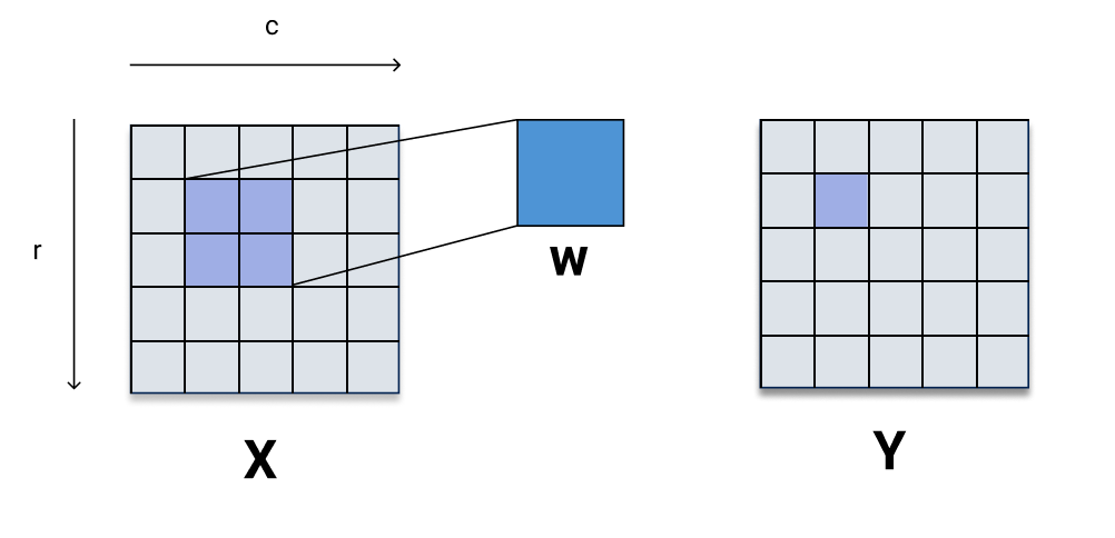
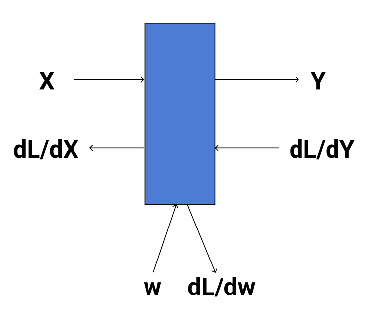
Recall in backprop at a given layer, we receive an upstream gradient $\frac{\partial L}{\partial \mathbf{y}}$ and we need to compute $\frac{\partial L}{\partial \mathbf{w}}$ and $\frac{\partial L}{\partial \mathbf{X}}$ for the backward pass.
Let’s start with $\frac{\partial L}{\partial \mathbf{w}}$.
Gradient of $\mathbf{w}$:
$\frac{\partial L}{\partial \mathbf{w}}$ is the same size as $\mathbf{w}$. We will consider computing the gradient at 1 entry in the kernel, i.e. $\frac{\partial L}{\partial \mathbf{w}[a’, b’]}$. We also have to incorporate the upstream gradient $\frac{\partial L}{\partial \mathbf{y}}$ that we are given. We can do this by asking the question: “how do slight changes to $\mathbf{w}[a’, b’]$ affect the output $\mathbf{y}$?”. Well, if we recall the forward pass, every pixel of $\mathbf{y}$ is a dot product of the kernel $\mathbf{w}$ with some region of the input, so small changes to $\mathbf{w}[a’, b’]$ will affect every pixel of the output! So we have
\[\begin{align*} \frac{\partial L}{\partial \mathbf{w}[a', b']} &= \sum_{p \in \mathbf{y}} \frac{\partial L}{\partial p} \frac{\partial p}{\partial \mathbf{w}[a', b']} \\ &= \sum_{r=0}^{N_{1}-1} \sum_{c=0}^{N_{2}-1} \frac{\partial L}{\partial \mathbf{y}[r, c]} \frac{\partial \mathbf{y}[r, c]}{\partial \mathbf{w}[a', b']} \end{align*}\]We already know $\frac{\partial L}{\partial \mathbf{y}[r, c]}$. To compute $\frac{\partial \mathbf{y}[r, c]}{\partial \mathbf{w}[a’, b’]}$ we can use the formula for the forward pass.
\[\begin{align*} \frac{\partial}{\partial \mathbf{w}[a', b']} \mathbf{y}[r, c] &= \frac{\partial}{\partial \mathbf{w}[a', b']} \sum_{a=0}^{k_{1}-1} \sum_{b=0}^{k_{2}-1} \mathbf{X}[r + a, c + b] \mathbf{w}[a, b] \\ &= \sum_{a=0}^{k_{1}-1} \sum_{b=0}^{k_{2}-1} \frac{\partial}{\partial \mathbf{w}[a', b']} \mathbf{X}[r + a, c + b] \mathbf{w}[a, b] \\ &= \mathbf{X}[r + a', c + b'] \end{align*}\]We can also arrive at the same conclusion by thinking about what pixel of $\mathbf{X}$ gets multiplied by $\mathbf{w}[a’, b’]$ when computing $\mathbf{y}[r, c]$. Visually:
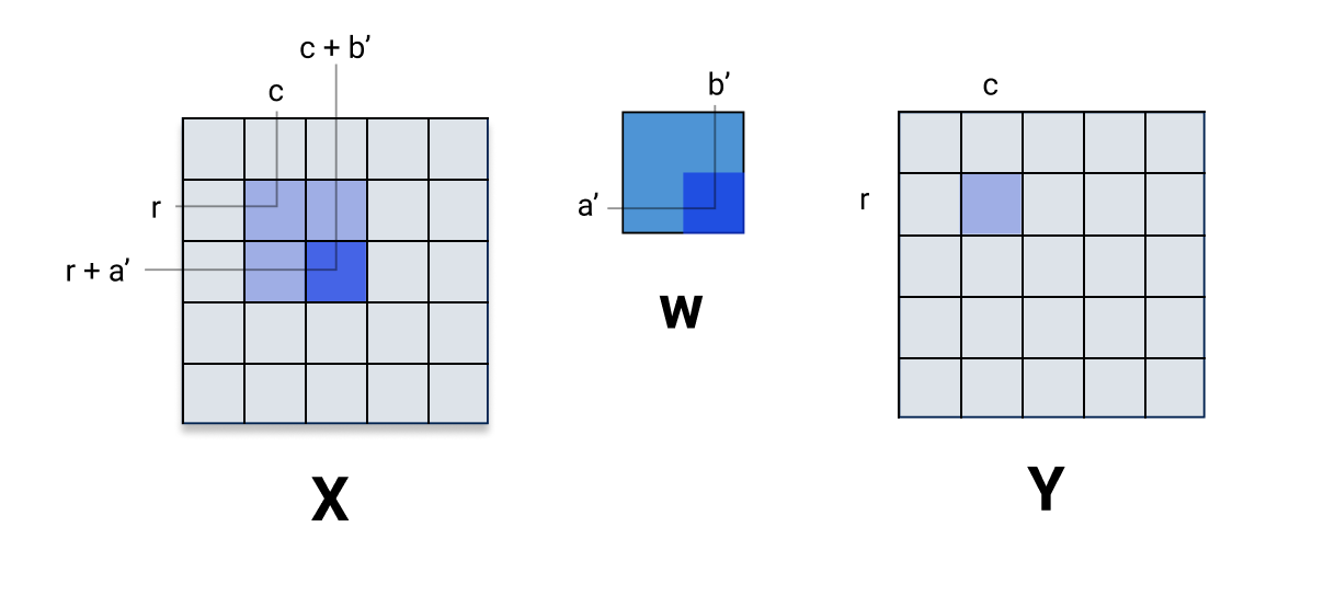
It should be clear that $\frac{\partial \mathbf{y}[r, c]}{\partial \mathbf{w}[a’, b’]} = \mathbf{X}[r + a’, c + b’]$. So, finally we have
\[\frac{\partial L}{\partial \mathbf{w}[a', b']} = \sum_{r=0}^{N_{1}-1} \sum_{c=0}^{N_{2}-1} \frac{\partial L}{\partial \mathbf{y}[r, c]} \mathbf{X}[r + a', c + b']\]So the gradient w.r.t. $\mathbf{w}$ is in fact a convolution between $\frac{\partial L}{\partial \mathbf{y}}$ and $\mathbf{X}$! Of course, since $\frac{\partial L}{\partial \mathbf{y}}$ and $\mathbf{X}$ are the same size, convolving them would yield a scalar, so it is actually a convolution with $\mathbf{X}$ padded such that the result of the convolution is size $k_{1} \times k_{2}$, because that is the size of $\frac{\partial L}{\partial \mathbf{w}}$.
\[\frac{\partial L}{\partial \mathbf{w}} = \mathbf{X}_{\text{padded}} * \frac{\partial L}{\partial \mathbf{y}}\]Gradient of $\mathbf{X}$:
Just like last time, let’s compute the gradient one pixel at a time. How do small changes to the pixel $\mathbf{X}[r’, c’]$ affect $\mathbf{y}$? Recall that one propety of convolutional layers is local connectivity, meaning a subset of the input is connected to a subset of the output (rather than dense connectivity in fully-connected layers). This means that $\mathbf{X}[r’, c’]$ is connected to some region in $\mathbf{y}$. How can we mathematically define this region?
As the kernel passes over $\mathbf{X}$, it passes over the pixel $\mathbf{X}[r’, c’]$ at some position and starts using it to compute output pixels. It passes over the pixel $\mathbf{X}[r’, c’]$ for the last time when computing output pixel $\mathbf{y}[r’, c’]$. Visually:
So computing the derivative w.r.t. $\mathbf{X}[r’, c’]$ amounts to summing over the region in $\mathbf{y}$ that depends on $\mathbf{X}[r’, c’]$. Let’s call that region $\mathbf{R}_{r’, c’} \subset \mathbf{y}$. From the image above, we can see
\[\mathbf{R}_{r', c'} = \mathbf{y}[\max(0, r' - k_{1} + 1) : r', \max(0, c' - k_{2} + 1) : c']\]And so,
\[\begin{align*} \frac{\partial L}{\partial \mathbf{X}[r', c']} &= \sum_{p \in \mathbf{R}_{r', c'}} \frac{\partial L}{\partial p} \frac{\partial p}{\partial \mathbf{X}[r', c']} \\ &= \sum_{a=0}^{k_{1}-1}\sum_{b=0}^{k_{2}-1} \frac{\partial L}{\partial \mathbf{y}[\max(0, r'-a), \max(0,c'-b)]} \frac{\partial \mathbf{y}[\max(0, r'-a), \max(0,c'-b)]}{\partial \mathbf{X}[r', c']} \end{align*}\]The max function prevents us from indexing out of bounds in $\mathbf{y}$. Let’s omit it for clarity, where it is understood that any negative index should be discarded. So we are left with
\[\frac{\partial L}{\partial \mathbf{X}[r', c']} = \sum_{a=0}^{k_{1}-1}\sum_{b=0}^{k_{2}-1} \frac{\partial L}{\partial \mathbf{y}[r'-a, c'-b]} \frac{\partial \mathbf{y}[r'-a,c'-b]}{\partial \mathbf{X}[r', c']}\]All that’s left is to compute $\frac{\partial \mathbf{y}[r’-a,c’-b]}{\partial \mathbf{X}[r’, c’]}$. We can do this analytically. Recall
\[\begin{align*} \mathbf{y}[r', c'] &= \sum_{\alpha=0}^{k_{1}-1} \sum_{\beta=0}^{k_{2}-1} \mathbf{X}[r' + \alpha, c' + \beta] \mathbf{w}[\alpha, \beta] \end{align*}\]So
\[\begin{align*} \mathbf{y}[r' - a, c' - b] &= \sum_{\alpha=0}^{k_{1}-1} \sum_{\beta=0}^{k_{2}-1} \mathbf{X}[r' - a + \alpha, c' - b + \beta] \mathbf{w}[\alpha, \beta] \\ \Rightarrow \frac{\partial}{\partial \mathbf{X}[r', c']} \mathbf{y}[r' - a, c' - b] &= \frac{\partial}{\partial \mathbf{X}[r', c']} \sum_{\alpha=0}^{k_{1}-1} \sum_{\beta=0}^{k_{2}-1} \mathbf{X}[r' - a + \alpha, c' - b + \beta] \mathbf{w}[\alpha, \beta] \\ &= \sum_{\alpha=0}^{k_{1}-1} \sum_{\beta=0}^{k_{2}-1} \frac{\partial}{\partial \mathbf{X}[r', c']} \mathbf{X}[r' - a + \alpha, c' - b + \beta] \mathbf{w}[\alpha, \beta] \\ &= \mathbf{w}[a, b] \end{align*}\]Now we can plug this result back into our equation for the derivative w.r.t. $\mathbf{X}[r’, c’]$.
\[\begin{align*} \frac{\partial L}{\partial \mathbf{X}[r', c']} &= \sum_{a=0}^{k_{1}-1}\sum_{b=0}^{k_{2}-1} \frac{\partial L}{\partial \mathbf{y}[r'-a, c'-b]} \frac{\partial \mathbf{y}[r'-a, c'-b]}{\partial \mathbf{X}[r', c']} \\ &= \sum_{a=0}^{k_{1}-1}\sum_{b=0}^{k_{2}-1} \frac{\partial L}{\partial \mathbf{y}[r'-a, c'-b]} \mathbf{w}[a, b] \end{align*}\]Closing Remarks
Hopefully this post was a helpful and concise explanation of backprop in conv layers. I am purposefully omitting code since that’s part of the homework for 7643. This is also good practice for defining the backward pass of other layers, which we will have to do a lot in CS 7643. Anyway, email me with questions, comments, passionate rants, and the like. Stay hydrated y’all.