Notes on Backpropagation in Convolutional Layers
29 December 2020
Revised 11 November 2023
This set of notes will discuss backpropagation in convolutional layers. We will derive the gradient of the loss with respect to the weights (kernel) and the input and discuss some interesting interpretations of these graidents. These notes were originially used for CS 7643: Deep Learning at Georgia Tech.
Preliminaries
First we will define some notation. We denote the input to the convolutional layer \( X \in \mathbb{R}^{H \times W} \), the output \( Y \in \mathbb{R}^{H' \times W'} \), and the parameters (i.e. the kernel) \( \Theta \in \mathbb{R}^{K \times K} \). For simplicity, we are assume there is no padding in the input, the kernel is square, and there is no channel dimension (i.e. there is one channel). We denote the scalar loss as \( L \).
We also use the notation of differentials and gradients interchangeably. For example, \( \nabla_{\Theta} L = \frac{\partial L}{\partial \Theta} \in \mathbb{R}^{K^2} \) is a vector of partial derivatives the same size as the flattened \( \Theta \).
Recall that in a convolutional layer, each feature in \( Y \) is computed as a cross-correlation of some region of \( X \) with \( \Theta \).
\[
\begin{equation}\label{eq:forward}
y_{h',w'} = \sum_{i=0}^{K-1} \sum_{j=0}^{K-1} x_{h'+i,w'+j} \theta_{i, j}
\end{equation}
\]
Also recall the basic API for the backward pass. We are given the upstream gradients from the next layer of the computation graph \( \nabla_{Y} L \) and return the gradients with respect to the parameters \( \nabla_{\Theta} L \) (used for gradient descent) and the with respect to the input \( \nabla_{X} L \) (used for continuing the backward pass).
Computing \( \nabla_{\Theta} L \)
We will now derive \( \nabla_{\Theta} L = \frac{\partial L}{\partial \Theta} \in \mathbb{R}^{K^2} \). Consider computing the gradient one entry at a time by considering the scalar \( \frac{\partial L}{\partial \theta_{i,j}} \). Logically we know that the parameter \( \theta_{i,j} \) contributes to every feature in the output, so we much incorporate the derivative of each of these features in our computation of \( \frac{\partial L}{\partial \theta_{i,j}} \). Using the chain rule we have:
\[
\begin{align*}
\frac{\partial L}{\partial \theta_{i,j}} &= \frac{\partial L}{\partial Y}\frac{\partial Y}{\partial \theta_{i,j}} \\
&= \sum_{h'=0}^{H'-1} \sum_{w'=0}^{W'-1} \frac{\partial L}{\partial y_{h',w'}}\frac{\partial y_{h',w'}}{\partial \theta_{i,j}}
\end{align*}
\]
We already have \( \frac{\partial L}{\partial y_{h',w'}} \) from the upstream gradient. To compute \( \frac{\partial y_{h',w'}}{\partial \theta_{i,j}} \), we can use Equation \( \ref{eq:forward} \).
\[
\begin{align*}
\frac{\partial}{\partial \theta_{i,j}} y_{h',w'} &= \frac{\partial}{\partial \theta_{i,j}} \sum_{i'=0}^{K-1} \sum_{j'=0}^{K-1} x_{h'+i',w'+j'} \theta_{i', j'} \\
&= x_{h'+i,w'+j}
\end{align*}
\]
This make sense because in the computation of \( y_{h',w'} \), \( \theta_{i,j} \) is only used once when it is multiplied by \( x_{h'+i,w'+j} \). So for each parameter \( \theta_{i,j} \) we have:
\[
\begin{equation}\label{eq:dLdTheta}
\frac{\partial L}{\partial \theta_{i,j}} = \sum_{h'=0}^{H'-1} \sum_{w'=0}^{W'-1} \frac{\partial L}{\partial y_{h',w'}} x_{h'+i,w'+j}
\end{equation}
\]
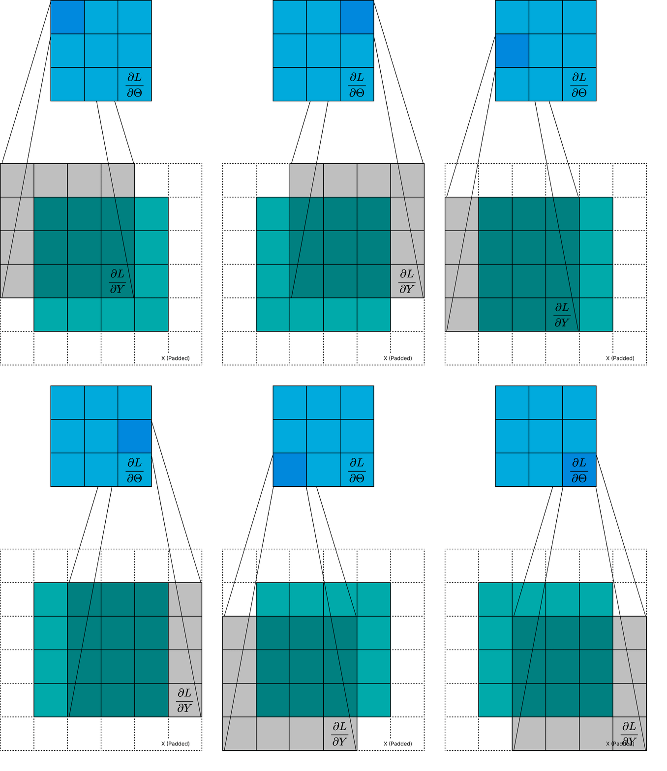
This can be thought of as one "pixel" of the gradient \( \frac{\partial L}{\partial \Theta} \). An interesting interpretation of Equation \( \ref{eq:dLdTheta} \) is that
the gradient \( \frac{\partial L}{\partial \Theta} \) is a cross-correlation between \( \frac{\partial L}{\partial Y} \) and the input \( X \). Actually, it is technically a cross-correlation using a padded version of \( X \) such that the output size is \( K \times K \).

Figure 1: Visualization of \( \frac{\partial L}{\partial \Theta} \) computation.
Computing \( \nabla_{X} L \)
Similarly, to compute \( \frac{\partial L}{\partial X} \in \mathbb{R}^{HW} \) we can consider one element \(\frac{\partial L}{\partial x_{h,w}}\) at a time and use the chain rule:
\[
\begin{align*}
\frac{\partial L}{\partial x_{h,w}} &= \sum_{h'=0}^{H'-1} \sum_{w'=0}^{W'-1} \frac{\partial L}{\partial y_{h',w'}}\frac{\partial y_{h',w'}}{\partial x_{h,w}}
\end{align*}
\]
Again, we have the upstream gradient \(\frac{\partial L}{\partial y_{h',w'}}\) and we can compute \(\frac{\partial y_{h',w'}}{\partial x_{h,w}}\) using Equation \( \ref{eq:forward} \).
\[
\begin{align*}
\frac{\partial}{\partial x_{h,w}} y_{h',w'} &= \frac{\partial}{\partial x_{h,w}} \sum_{i=0}^{K-1} \sum_{j=0}^{K-1} x_{h'+i,w'+j} \theta_{i, j} \\
&= \theta_{h-h',w-w'}
\end{align*}
\]
where the last line follows from the fact that \( x_{h,w} \) only appears where \( i = h - h' \) and \( j = w - w' \). Now we have:
\[
\begin{equation}\label{eq:dLdX}
\frac{\partial L}{\partial x_{h,w}} = \sum_{h'=0}^{H'-1} \sum_{w'=0}^{W'-1} \frac{\partial L}{\partial y_{h',w'}} \theta_{h-h',w-w'}
\end{equation}
\]
Remark: Of course, when either index of \( \theta_{h-h',w-w'} \) is out of bounds of the kernel dimensions, we omit the term from the summation. This is equivalent to the case where the input pixel \( x_{h,w} \) is not used in the computation of the output \( y_{h',w'} \) because the kernel is not covering that region of the input. Therefore, the summation only includes up to \( K^2 \) valid terms.
Using the above remark and the equations \( i = h - h', j = w - w' \), we can write Equation \( \ref{eq:dLdX} \) equivalently as
\[
\begin{equation}
\frac{\partial L}{\partial x_{h,w}} = \sum_{i=0}^{K-1} \sum_{j=0}^{K-1} \frac{\partial L}{\partial y_{h-i,w-j}} \theta_{i,j}
\end{equation}
\]
Interestingly,
the full gradient \( \frac{\partial L}{\partial X} \) can be thought of as a cross-correlation between a padded version of \( \frac{\partial L}{\partial Y} \) and the kernel \( \Theta \).
